Use of super-site observations to evaluate near-surface temperature forecasts
Polly Schmederer, Irina Sandu, Thomas Haiden, Anton Beljaars, Martin Leutbecher (all ECMWF), Claudia Becker (DWD, Germany)
Systematic forecast errors in temperature and humidity near the surface can be better understood by also examining errors higher up in the atmospheric boundary layer and in the soil. Meteorological observatories, also known as super-sites, provide long-term observational records of such vertical profiles and of surface energy budget components, such as surface radiative fluxes. Those datasets thus constitute an invaluable resource for ECMWF’s efforts to further reduce forecast errors in near-surface weather parameters. Initial findings for 2‑metre temperature errors in ECMWF forecasts at two European super-sites suggest that the errors are partly the result of the model exchanging too much energy between the atmosphere and the land. However, the influence of other factors, such as errors resulting from the representation of vegetation in semi-arid areas and from small-scale variations in vegetation and soil type near measurement stations, mean that it is difficult to adjust the energy exchange in a way which leads to an overall error reduction on the European scale.
Increasing use of super-sites
ECMWF verifies forecasts of 2‑metre temperature (T2m) and 2‑metre dew point (D2m) against observations from SYNOP weather stations on a routine basis. These evaluations reveal that forecast biases undergo annual and diurnal variations and exhibit large-scale geographical patterns. Biases in T2m and D2m can be due to a multitude of factors, such as the representation of the surface physiography (including vegetation, soil type, soil texture), soil temperature, soil moisture, atmospheric mixing, strength of land–atmospheric coupling, cloud cover, cloud properties and wind speed.
The routine verification against SYNOP observations does not provide information about forecast errors within the lower atmosphere, in the soil or at their interface. In a recent project focused on ‘Understanding uncertainties in surface–atmosphere exchange’ (USURF), ECMWF started to use data from super-sites such as Falkenberg (Germany, associated with Meteorologisches Observatorium Lindenberg – Richard-Aßmann-Observatorium), Cabauw (the Netherlands) and Sodankyla (Finland) more systematically than before to evaluate the quality of forecasts in the lowest part of the atmosphere (up to 100 m) and in the soil/snow, in an attempt to disentangle sources of forecast error in near-surface weather parameters. Such observations have been used previously at ECMWF to investigate wind errors (see Sandu et al., 2014).
Systematic errors in near-surface temperature
The focus of this article is on the use of super-site observations from Falkenberg and Cabauw (Box A) to evaluate ECMWF high-resolution deterministic (HRES) and ensemble (ENS) forecasts for the 12-month period from June 2017 to May 2018. The super-sites are in regions without complex topography. Unlike Cabauw, Falkenberg has the additional advantage of being situated inland, so that coastal effects play no role. Such conditions are ideal for capturing large-scale error patterns instead of local meteorological effects. This is why the analysis presented here largely focuses on Falkenberg. The German National Meteorological Service (DWD) kindly provides the observational data on a daily basis in near-real time. It has also provided forecasts from their global Icosahedral Nonhydrostatic Model (ICON) for a selected period. The Royal Netherlands Meteorological Institute (KNMI) kindly provides the observations at Cabauw.
A
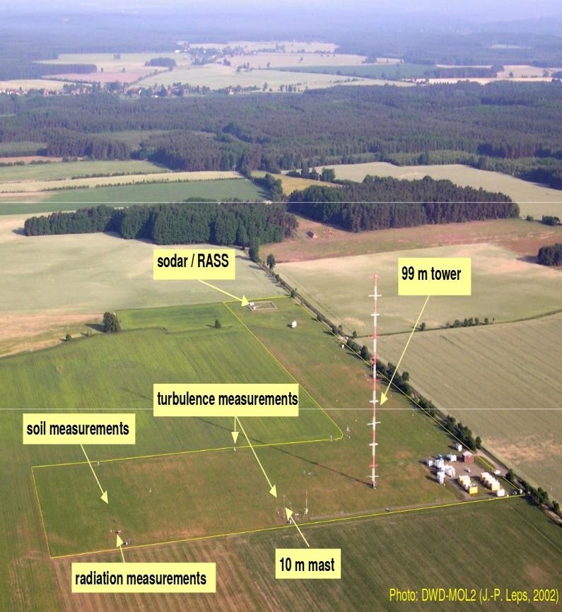
The Falkenberg and Cabauw super-sites
Falkenberg
Coordinates: 52.17°N, 14.12°E at an elevation of 73 m above mean sea level.
Observations include surface, soil, atmospheric and flux measurements every 10 minutes.
The tower has a height of 98 m. Soil measurements are made to a depth of 1.5 m.
The super-site is located in a rural area with open fields close to the site and patches of forest nearby.
The ground consists of sandy soils on top of a layer of loam, which is typically at a depth of 50–80 cm.
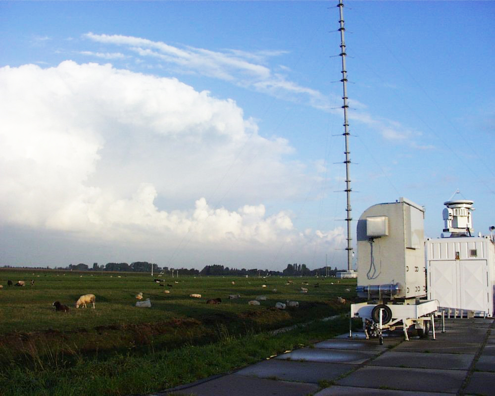
Coordinates: 51.971°N, 4.927°E at an elevation of 0.7 m below mean sea level.
The North Sea is at a distance of 50 km to the west-northwest.
Observations include surface, soil, atmospheric and flux measurements every 10 minutes.
The tower has a height of 217 m. Soil measurements are made to a depth of 0.5 m.
The super-site is located in agricultural grassland with open land to the west, windbreaks to the east, and mixed land (pastures and some windbreaks) to the north and south.
The ground consists of 0.6 m of river clay above a thick layer of peat.
Within the June 2017 to May 2018 period, we focus here on the summer months (June, July and August) since in this season the amplitude of the diurnal cycle of T2m is substantially underestimated in ECMWF forecasts (see Haiden et al., 2018). The night-time minimum temperature (Tmin) is typically 1–2 K too high in HRES forecasts and the day-time maximum temperature (Tmax) 1–2 K too low. This issue is present in the land areas of the extratropics for Tmin and in land areas across the globe for Tmax (Figure 1) and its causes need to be better understood. The mean error (bias) shown in Figure 1 is based on a subset of SYNOP stations. It includes only stations where the model orography differs by no more than 100 m from the actual terrain elevation, and where at least three of the four nearest grid points are land points. This is to exclude locations where the model cannot be expected to provide bias-free forecasts simply due to limitations imposed by horizontal resolution. The purpose of this filtering is the same as the selection of the super-sites: to capture mainly large-scale bias patterns and reduce the impact of local effects on evaluation results.
%3Cstrong%3E%20Figure%201%E2%80%82%3C/strong%3E%20Mean%20error%20(bias)%20of%20(a)%C2%A0daily%20minimum%20T2m%20(Tmin)%20and%20(b)%C2%A0daily%20maximum%20T2m%20(Tmax)%20for%20a%20forecast%20range%20of%2072%20to%2096%C2%A0hours%20in%20summer%202017%20(June,%20July%20and%20August).%20Verification%20is%20against%20SYNOP%20observations.%20Stations%20for%20which%20the%20model%20elevation%20differs%20by%20more%20than%20100%C2%A0m%20from%20the%20true%20elevation%20and%20stations%20where%20the%20nearest%20grid%20point%20is%20a%20sea%20point%20were%20not%20included.%20 Figure 1 Mean error (bias) of (a) daily minimum T2m (Tmin) and (b) daily maximum T2m (Tmax) for a forecast range of 72 to 96 hours in summer 2017 (June, July and August). Verification is against SYNOP observations. Stations for which the model elevation differs by more than 100 m from the true elevation and stations where the nearest grid point is a sea point were not included.
T2m is a diagnostic variable in ECMWF’s Integrated Forecasting System (IFS), which means that it is not predicted directly by the model but is derived from other variables. Specifically, it is computed through vertical interpolation between the temperature at the lowest model level (about 10 m above the surface) and the surface (or skin) temperature. Biases can stem from biases in skin or air temperature or they can be due to the profile function used to derive the T2m diagnostic. To better understand and identify the sources of the errors, it is useful to look at the observed and predicted profiles of temperature in the atmosphere and soil at Falkenberg. Figure 2 shows such profiles for 4-day HRES, ENS mean and ICON forecasts and for observations. It shows that, at 00 UTC, the HRES is too warm not only at 2 m but also at the surface and in the lowest part of the atmosphere up to 20 m. Above 35 m, the HRES is too cold since here the night-time inversion (warmer temperatures at greater heights) is not sufficiently pronounced. In the soil, the HRES is too cold at all depths. The fact that the biases are not confined to 2 m suggests that they are due not only to the computation of the T2m diagnostic but also to the representation of the prognostic (i.e. directly predicted) temperatures at the surface, within the atmosphere or in the soil. DWD’s ICON is also too warm at, and close to, the surface, but above 60 m it matches observations well for the selected period. In the soil, ICON is too cold in the first soil layer and matches observations well in deeper soil layers.
%3Cstrong%3E%20Figure%202%E2%80%82%3C/strong%3E%20Observed%20and%20predicted%20profiles%20of%20(a)%C2%A0air%20temperature%20and%20(b)%C2%A0soil%20temperature%20at%20Falkenberg.%20The%20forecasts%20are%20for%20day%C2%A04%20at%2000%C2%A0UTC%20and%20are%20averaged%20over%20the%20summer%C2%A02017%20(June,%20July%20and%C2%A0August). Figure 2 Observed and predicted profiles of (a) air temperature and (b) soil temperature at Falkenberg. The forecasts are for day 4 at 00 UTC and are averaged over the summer 2017 (June, July and August).
Systematic errors of medium-range ensemble forecasts were examined too. The ensemble mean behaves similarly to the HRES, being too warm at 2 m and at the surface, and too cold in the soil (Figure 2). For the study period, only the surface parameters were available for the ensemble forecasts, since model level data are not operationally archived. Recently we started to extract data on model levels at the super-sites from the ensemble forecasts for the Boundary Conditions programme, which stores the whole profile of the ensemble forecasts for a limited period of time. In the future, this will make it possible to also assess ensemble forecast errors in the lower atmosphere at the super-sites.
To get a better idea of the temporal evolution of the forecast biases at Falkenberg, monthly averaged diurnal cycles of temperature at different heights in the atmosphere (surface, 2 m, 10 m, 98 m), and different depths in the soil (5 cm, 20 cm, 60 cm) are shown in Figure 3. Both in HRES and ICON, the amplitude of the diurnal cycle is underestimated in the atmosphere, with larger biases close to the surface. During the night, in both models the temperatures are about 1–2 K too warm at 2 m and about 2 K too warm at the surface. HRES slightly overestimates the diurnal cycle of the soil temperature in the first soil layer, being up to 2 K too cold at night. In all other soil layers, the HRES is too cold at all times. ICON is warmer than the IFS in all soil layers during the day, and slightly colder during the night, which leads to a slightly stronger overestimation of the diurnal cycle. The ensemble mean behaves similarly to the HRES and therefore has the same systematic error.
%3Cstrong%3E%20Figure%203%E2%80%82%3C/strong%3E%20Monthly%20averaged%20diurnal%20cycles%20of%20temperatures%20at%20(a)%C2%A0different%20heights%20in%20the%20air%20and%20(b)%C2%A0different%20depths%20in%20the%20soil%20at%20Falkenberg%20at%20forecast%20day%C2%A04%20for%20the%20months%20of%20June,%20July%20and%20August%C2%A02017. Figure 3 Monthly averaged diurnal cycles of temperatures at (a) different heights in the air and (b) different depths in the soil at Falkenberg at forecast day 4 for the months of June, July and August 2017.Too much heat transfer?
The results shown in Figures 2 and 3 suggest that ICON and the IFS have similar systematic errors in the atmosphere and in the soil close to the surface but exhibit different behaviour in the deeper soil. The main conclusion from the diurnal cycle evaluation for the summer period is that probably too much energy is exchanged between the atmosphere and the land, especially for the IFS. This means, for example, that during the night too much energy is extracted from the soil and transferred to the atmosphere. This results in soil temperatures that are too cold and skin temperatures and T2m that are too warm. The same qualitative behaviour can be observed at Cabauw (not shown).
The parameter that controls the heat transfer between the vegetation layer and the soil is the skin layer conductivity λskin. In the IFS, the values of this parameter were reduced for some vegetation types in the upgrade to IFS Cycle 43r1 implemented in November 2016. This led to a slight improvement in T2m forecasts. The Falkenberg evaluation suggests, however, that these values are perhaps still too high.
A sensitivity experiment (EXP) has been performed to test this hypothesis. It has been carried out for the short range only (up to 48 h) to minimize feedback effects from the large-scale flow and isolate the direct impact of the physics changes. λskin was further reduced from 10 to 5 W m-2 K-1 for the vegetation types ‘crops’ (low vegetation) and ‘interrupted forest’ (high vegetation), which are the dominant vegetation types in the IFS in the Falkenberg area, as well as in Europe in general. As expected, this adjustment compared to the operational setup (CTR) reduced the night-time T2m and skin temperature at Falkenberg and Cabauw on average by about 1 K and 0.5 K, respectively. It also cooled the temperature in the first soil layer at day-time by 1 K and 0.5 K in Falkenberg and Cabauw, respectively (not shown), but had little response at night-time in the soil. The T2m biases were thus almost halved at Falkenberg and almost entirely removed on average over the 3‑month summer period at Cabauw, where the biases are smaller. On the European scale, the impact of this reduction in thermal coupling varies. At day-time, the effect is small and there is almost no change in bias (Figure 4a,c). At night-time, in the continental region over eastern Europe, characterised by a big systematic warm bias at night, the reduction in thermal coupling reduces the T2m error (Figure 4b,d). In parts of western Europe where the bias is smaller and more variable, e.g. over Germany and the Iberian Peninsula, the change seems to be too big and results in a predominantly cold bias (Figure 4d). On average, reducing λskin does not have a positive effect on T2m forecast performance on the European scale, leading to smaller biases at some stations, but larger biases at others. This is very likely due to the fact that these biases are partly due to other factors than the thermal land–atmosphere coupling. One of these other factors is likely the representation of vegetation in semi-arid areas, where low vegetation potentially dies in summer. The model does not capture this effect, and water from the low vegetation keeps evaporating, which cools the surface during the day. During the night, the model vegetation insulates the soil more effectively than the vegetation does in reality, which may contribute to the night-time warm bias. Another potential issue is heterogeneity. The model assumes homogeneity in regions where in reality vegetation and soil types vary on small scales or the dominant soil and vegetation type are not representative for the measurement station.
%3Cstrong%3E%20Figure%204%E2%80%82%3C/strong%3E%20Mean%20error%20of%20T2m%20at%20forecast%20day%C2%A02%20at%20(a)%C2%A012%C2%A0UTC%20with%20operational%20land%E2%80%93atmosphere%20coupling%20(CTR),%20(b)%C2%A000%C2%A0UTC%20with%20operational%20land%E2%80%93atmosphere%20coupling%20(CTR),%20(c)%C2%A012%C2%A0UTC%20with%20decreased%20land%E2%80%93atmosphere%20coupling%20(EXP),%20and%20(d)%C2%A000%C2%A0UTC%20with%20decreased%20land%E2%80%93atmosphere%20coupling%20(EXP).%20Verification%20was%20performed%20against%20the%20same%20subset%20of%20SYNOP%20observations%20as%20in%20Figure%C2%A01. Figure 4 Mean error of T2m at forecast day 2 at (a) 12 UTC with operational land–atmosphere coupling (CTR), (b) 00 UTC with operational land–atmosphere coupling (CTR), (c) 12 UTC with decreased land–atmosphere coupling (EXP), and (d) 00 UTC with decreased land–atmosphere coupling (EXP). Verification was performed against the same subset of SYNOP observations as in Figure 1.
Reliability of ensemble forecasts
The ensemble provides flow-dependent estimates of forecast uncertainty. One interesting question is how reliably the ensemble spread reflects the magnitude of the error of the ensemble mean. Following the approach described by Yamaguchi et al. (2016), the reliability of the ensemble spread was examined by sorting the forecast–observation pairs by increasing ensemble variance into five equally populated classes. Variations in the expected magnitude of the random error are captured rather well by the ensemble for T2m forecasts at day 4 at Falkenberg. Figure 5 shows the relationship between the variance and the mean squared error of the ensemble mean for forecast day 4. Even the raw data are a good fit to the diagonal that represents a perfectly reliable ensemble. Removing the systematic error from the ensemble mean (bias correction) improves the fit. When verifying with observations, the observation uncertainty needs to be accounted for by adding an estimate of the observation error variance to the ensemble variance. We use a value of 1 K2 as an estimate for the T2m observation error variance. This value is similar to the estimate used in the data assimilation system for radiosonde temperature observations in the lower troposphere. Accounting for the observation error variance has an even bigger positive effect than correcting for the systematic bias. Combining both corrections yields an almost perfect relationship for T2m in summer. Therefore, there is no evidence of an underdispersion of the ensemble. We conclude that the systematic error (Figure 3) is the main issue for T2m in the medium-range forecast of the ensemble in Falkenberg at day 4. Further investigations are ongoing to analyse different lead times and locations as well as the profile of the lower atmosphere and the soil for a deeper understanding of T2m forecast errors.
%3Cstrong%3E%20Figure%205%E2%80%82%3C/strong%3E%20Reliability%20diagrams%20for%20ENS%202%E2%80%91metre%20temperature%20forecasts%20for%20Falkenberg%20at%20forecast%20day%C2%A04%20in%20June,%20July%20and%20August%C2%A02017.%20To%20create%20the%20charts,%20three-hourly%20data%20were%20grouped%20into%20five%20equally%20populated%20classes%20of%20increasing%20ensemble%20variance.%20The%20mean%20ensemble%20variance%20and%20the%20mean%20squared%20ensemble%20mean%20error%20were%20then%20computed%20for%20each%20class%20(i)%C2%A0with%20the%20raw%20data;%20(ii)%C2%A0with%20raw%20ensemble%20data%20but%20accounting%20for%20observation%20errors;%20(iii)%C2%A0with%20bias-corrected%20ensemble%20data%20but%20raw%20observations;%20and%20(iv)%C2%A0with%20bias-corrected%20ensemble%20data%20and%20accounting%20for%20observation%20errors. Figure 5 Reliability diagrams for ENS 2‑metre temperature forecasts for Falkenberg at forecast day 4 in June, July and August 2017. To create the charts, three-hourly data were grouped into five equally populated classes of increasing ensemble variance. The mean ensemble variance and the mean squared ensemble mean error were then computed for each class (i) with the raw data; (ii) with raw ensemble data but accounting for observation errors; (iii) with bias-corrected ensemble data but raw observations; and (iv) with bias-corrected ensemble data and accounting for observation errors.
Spatial representativeness
When point observations are used for verification, the question of representativeness arises. Even in the absence of significant topography, the Earth’s surface exhibits substantial inhomogeneities due to variations in vegetation cover and soil type. Thus, an assessment is required of how representative the results of the super-site evaluation are at grid-box scale and beyond. The ‘representativeness error’ can be defined as the difference between a ‘grid-box mean’ observed value and the point observations. The true grid-box mean observed value is not known but we can obtain an estimate by upscaling T2m observations (i.e. averaging over SYNOP stations within a certain area). Differences in elevation between stations are taken into account using the standard 0.0065K/m temperature gradient. Figure 6 shows such an estimation of representativeness errors for central Europe for 20 km grid boxes in terms of the absolute value of the mean difference (|BIAS|) and the root-mean-square difference (RMSD). As expected, representativeness errors are generally larger at night, and the bias makes a substantial contribution to the RMSD. Somewhat surprisingly, representativeness errors are smallest in winter. This appears to be due to the (on average) higher wind speeds in that season, which reduce small-scale inhomogeneities in the temperature field other than those connected to elevation. Results like those shown in Figure 6 provide a benchmark for the IFS, indicating the minimum level of forecast error that can be expected at the given horizontal resolution.
%3Cstrong%3E%20Figure%206%E2%80%82%3C/strong%3E%20Estimation%20of%20T2m%20representativeness%20error%20at%2000%C2%A0UTC%20and%2012%C2%A0UTC%20based%20on%20SYNOP%20observations%20in%20central%20Europe%20(48%E2%80%9355%C2%B0N,%206%E2%80%9315%C2%B0E)%20in%20the%20period%202016%E2%80%932018.%20The%20chart%20shows%20the%20absolute%20value%20of%20the%20bias%20(%7CBIAS%7C)%20and%20the%20root-mean-square%20difference%20(RMSD)%20between%20the%20point%20observations%20and%20the%20mean%20observed%20value%20within%2020x20%C2%A0km%20boxes.%20 Figure 6 Estimation of T2m representativeness error at 00 UTC and 12 UTC based on SYNOP observations in central Europe (48–55°N, 6–15°E) in the period 2016–2018. The chart shows the absolute value of the bias (|BIAS|) and the root-mean-square difference (RMSD) between the point observations and the mean observed value within 20x20 km boxes.
Outlook
Super-site observations have become a valuable additional resource for further developing parametrizations of boundary-layer processes and of surface–atmosphere exchange. They make it possible to gain deeper insights into possible causes of biases in near-surface weather parameters. However, when used for evaluation studies, their limitations in terms of horizontal representativeness must be kept in mind. The complicated patterns of cold/warm biases both at global and European scale, as for example illustrated by Figure 4a, are not fully understood and need to be further investigated. It would be interesting to explore whether more up-to-date mapping of the vegetation, land use, or soil properties could help to address some of these errors in near-surface temperature or humidity. Other possible areas of investigation are how these errors are affected by the modelling of mixing within the atmospheric boundary layer or of heat transfer within the soil. For example, the choice of soil vertical discretisation and the total depth of soil represented in the IFS (currently 2.89 m) can affect the thermal diffusivity (rate of heat transfer) with an impact on deep soil temperature biases. Preliminary investigations suggest that the thermal diffusivity in the model is fairly similar at Falkenberg and Cabauw, while that derived from observations, using a method similar to that described by Verhoef et al. (1996), is quite different. One reason for this could be that the soil types at the two sites are quite different, with sandy soil at Falkenberg, and river clay at Cabauw. Overall, further reductions in near-surface biases in the IFS appear possible but will require both systematic modelling efforts and a quantitative assessment of the representativeness of observations at the locations of SYNOP stations and super-sites.
Further reading
Haiden, T., I. Sandu, G. Balsamo, G. Arduini & A. Beljaars, 2018: Addressing biases in near-surface forecasts. ECMWF NewsletterNo. 157, 20–25.
Sandu, I., A. Beljaars & G. Balsamo, 2014: Improving the representation of stable boundary layers. ECMWF NewsletterNo. 138, 24–29.
Yamaguchi, M., S.T.K. Lang, M. Leutbecher, M. J. Rodwell, G. Radnoti & N. Bormann, 2016: Observation‐based evaluation of ensemble reliability. Q. J. R. Meteorol. Soc., 142, 506–514.
Verhoef, A., B. van der Hurk, A. Jacobs & B. Heusinkveld, 1996: Thermal soil properties for vineyard (EFEDA-I) and savanna (HAPEX-Sahel) sites. Agricultural and Forest MeteorologyNo. 78, 1–18.