
Machine learning and deep learning (ML/DL) techniques have made remarkable advances in recent years in a large and ever-growing number of disparate application areas, such as natural language processing, computer vision, autonomous vehicles, healthcare, finance and many others. These advances have been driven by the huge increase in available data, the corresponding increase in computing power and the emergence of more effective and efficient algorithms. In Earth sciences in general, and numerical weather prediction (NWP) and climate prediction in particular, ML/DL uptake has been slow at first, but interest is rapidly growing. Today innovative applications of standard ML/DL tools and ideas are becoming increasingly common, and ECMWF has recently set out its approach in a ‘roadmap for the next 10 years’ (Düben et al., 2021).
The interest of Earth scientists in ML/DL techniques stems from different perspectives. On the observation side, for example, the current and future availability of satellite-based Earth system measurements at high temporal and spatial resolutions and the emergence of entirely new observing systems made possible by ubiquitous internet connectivity (the so‑called ‘Internet of Things’) pose new challenges to established processing techniques and ultimately to our ability to make effective use of these new sources of information. ML/DL tools can potentially be useful to overcome some of these problems, for example in the areas of observation quality control, observation bias correction and the development of efficient observation operators.
ML/DL approaches are also interesting from the point of view of data assimilation, in other words the combination of the latest observations with a short-range forecast to obtain the best possible estimate of the current state of the Earth system. This is because such approaches can be typically framed as Bayesian estimation problems which make use of a similar methodological toolbox to the one used in variational data assimilation. This fact has been recognised in the new ECMWF Strategy 2021–2030, which acknowledges that “4D‑Var data assimilation is uniquely positioned to benefit from integrating machine learning technologies because the two fields share a common theoretical foundation and use similar computational tools”. It is apparent that some of the techniques already widely adopted in the data assimilation community (e.g. model error estimation, model parameter estimation, variational bias correction) are effectively a type of ML algorithm. The question is then, what lessons can the NWP/climate prediction community learn from the methodologies and practices of the ML/DL community? How can we seamlessly develop the ML/DL techniques already used in the NWP/climate prediction workflow and integrate new ideas into current data assimilation practices?
In this article we briefly discuss the underlying theoretical equivalence between today’s data assimilation and modern ML/DL. We then provide some concrete examples of how the adoption of ML/DL ideas in the NWP workflow has the potential to extend the capabilities of current data assimilation methodologies and ultimately lead to better analyses and forecasts.
Machine learning: a form of data assimilation
The aims of data assimilation and machine learning are similar: to learn about the world using observations. In traditional weather forecasting we assume we have a reasonably accurate physical model of the Earth system, and the biggest unknown is the initial conditions from which to start the forecast. In machine learning the physics is unknown, and the aim is to learn an empirical model directly from the observations. In both fields, Bayes’ theorem provides an underlying description of how to incorporate information from observations. This gives a way of mathematically comparing the two approaches.
Rather than show the equations, Figure 1 gives the Bayesian network diagram for both approaches (Geer, 2021). The black text represents data assimilation, such as the 4D‑Var system used in ECMWF’s Integrated Forecasting System (IFS). The arrows together represent the action of the forecast model and observation operator, which take the model state of the Earth system (x) and the parameters of the physical model (w) and provide estimates of the observations (y). By comparing these estimates to real observations, data assimilation finds a better estimate of the initial conditions (x). In the IFS, we do not yet try to improve the parameters of the model at the same time. Such a process is known as parameter estimation and it is routinely done in fields like chemical source inversion or groundwater modelling. However, we already estimate some parameters in 4D‑Var: this is done in the weak-constraint term, which corrects model bias in the stratosphere, and in variational bias correction, which corrects observational bias. Research on estimating model parameters in the IFS is only just starting and is an exciting prospect (see later).

In a typical form of machine learning like a neural network, the training is done between data pairs, known as features (x) and labels (y). These are shown in blue text in Figure 1. A feature might be a picture, the label might be ‘cat’. A neural network is trained on a huge set of labelled features, with the aim to estimate weights (w) for a neural network. The trained network can then be used, in this example to identify animals in pictures. But the technique is very flexible, and applications range from playing games with higher skill than the best human players to learning to translate from one language to another.
The Bayesian network in Figure 1 is a mathematical abstraction, but by making a few assumptions we can get to the usual forms of variational data assimilation and machine learning, both of which minimise a cost function (known as a loss function in machine learning) to find the best x or w, or both (see Box A). The minimisation of the cost function in machine learning is usually done through a process called ‘back-propagation’. The same process takes place in data assimilation when we calculate the gradient of the cost function using the adjoint of the observation operator and the forecast model. As shown in the box, there is a mathematical equivalence between the processes of machine learning and those of variational data assimilation.
A
The aim of variational data assimilation or the training phase in machine learning is to reduce the cost function J(x,w) as much as possible by varying x and w. Here x and w are as defined in Figure 1, in other words state and parameters in data assimilation, or features and weights in machine learning:

The minimum of J(x,w) gives the maximum likelihood estimate of x and w. To find this, we must reduce the misfit between the model-simulated observations (or the neural-network simulated labels) and the real observations, which is measured by the observation term in the cost function, Jy, while not increasing the other terms in the cost function too much. Here y is the observation value and h(x,w) represents either the neural network or the physical model (including observation operator) in 4D-Var. For simplicity all the variables are scalars. Data assimilation weighs the observations according to their accuracy, here shown by the observation error standard deviation σy. Machine learning does not explicitly represent the observation error, but the process of data preprocessing (quality control, batch normalisation) can represent some (but not all) sources of observational uncertainties. The Jx term is what we call the background term in 4D-Var, with xb being the background forecast and σx the background error. This has no equivalent in machine learning, which assumes the features (e.g. the cat pictures) are free from error. The final term, Jw, constrains the estimated weights. In data assimilation, there are background estimates for the parameters, wb, which have an error σw. In machine learning, the equivalent is ridge regression, which regularises the weights, but the background weight estimate is 0 and its error standard deviation is 1.
One big advantage of data assimilation is that it can incorporate constraints from prior knowledge, such as the physics of the atmosphere, which helps provide a more accurate result than can be learnt solely from the observations. There is now a rapid development of ‘physically constrained’ machine learning approaches, but we might wonder if the end result will be to re-invent data assimilation. Machine learning’s strength is to operate in areas where there is scarce or no existing physical knowledge to constrain the solution – for example, there is no rule-based algorithm available for translating from one language to another. Within data assimilation for weather forecasting, the obvious place to use machine learning is also where we lack physical knowledge. This leads to some of the examples in this article, which explore learning the patterns of bias in the forecast model or in the observations, where this is hard to understand by purely physical reasoning. The highly accessible software tools provided by the machine learning community have made it easy to get started. A second scenario is where we might be reasonably confident in the equations of the physical system, but the parameters, such as roughness length in the boundary layer turbulence scheme, are not well known and may vary geographically on fine scales. This is probably better done using parameter estimation within the existing data assimilation framework. Another big application area for machine learning, which is not covered here, is not directed at improving the models but instead to produce faster statistical models from existing, slower and more computationally demanding physical models (i.e. model emulation).
Model error estimation and correction
ECMWF continues to make good progress in driving down model error, which together with initial uncertainties is one of the main obstacles to improved accuracy and reliability of weather and climate predictions. However, realistically there will always be some residual error. Recent advances in the context of weak-constraint 4D‑Var showed that it is possible to estimate and correct for a large fraction of systematic model error which develops in the stratosphere over short forecast ranges (Laloyaux & Bonavita, 2020). In each data assimilation cycle, weak-constraint 4D‑Var (WC-4DVar) optimises the fit of the short-range forecast trajectory to observations in two ways: by suitably changing the initial conditions (as in strong-constraint 4D‑Var), and by suitably adjusting a forcing term in the model equations to correct for the model error over the assimilation window.
An Artificial Neural Networks (ANNs) approach has been recently investigated as a way to predict the analysis increments by means of ML/DL. The systematic component of those increments can be viewed as another estimate of the cumulated model error over the assimilation window (Bonavita & Laloyaux, 2020). A set of climatological predictors is selected (latitude, longitude, time of day, month) to capture the part of model error which is related to geographical location, the diurnal cycle, and the seasonal cycle. State predictors are also used to represent the part of model error linked to the large-scale state of the flow, for example in oceanic stratocumulus areas, the Intertropical Convergence Zone, and extratropical cyclonic areas. To produce the input and the target of the neural network dataset, these predictors were extracted from the operational first guess and analysis increment for mass, wind, and humidity over the whole year 2018. Fully connected ANNs with multiple hidden nonlinear layers are trained and then used to produce model error tendencies over August 2019. These tendencies are applied to the model equations similarly to what is done in weak-constraint 4D‑Var. The plot in Figure 2 compares the temperature model error estimates from ANN and from weak-constraint 4D‑Var (applied only in the stratosphere at the moment).

WC‑4DVar corrects the warm bias in the upper stratosphere and the cold bias in the mid/lower stratosphere. It correctly captures the transition layer (20 to 10 hPa) where the model bias changes from cold to warm. The transition level between the cold and the warm bias layers is estimated at the same pressure level by the ANN. The main difference is in the upper stratosphere, where the neural network produces a positive correction of around 2 hPa. This is because this signal is present in the analysis increments used to train the neural network. On the other hand, WC‑4DVar extrapolates the cold bias to the top of the model, due to the deep vertical structure of the prescribed model error covariance matrix.
WC-4DVar is an online example of a statistical estimation technique as the algorithm updates the model error correction after each assimilation window. The current ANN produces a static correction dataset computed prior to the assimilation of the observations, but work is ongoing to apply the ANN online in a 4D‑Var system. In this context, the neural network will be applied in every assimilation window to the actual first-guess trajectory, instead of being applied offline to the pre-computed first-guess trajectories of the operational suite.
Model parameter estimation
Parameter estimation is widely used to make a model better fit a target. From this perspective, parameter estimation techniques can be considered as machine learning techniques. Estimating model parameters as part of a data assimilation process has been little studied so far. In such a framework, the parameters are re-estimated at each assimilation cycle using present information and past accumulated knowledge on the parameter.
The ability to estimate a parameter within the IFS 4D‑Var was demonstrated a few years ago with the estimation of the solar constant, which is a model parameter constrained indirectly by satellite observations. We are currently testing this idea on the sub-grid scale orography parametrization, which is a component of the physical parametrizations with a significant impact on the surface pressure field. The standard deviation of sub-grid orography is well known as a key variable of the sub-grid scale orography parametrization. As a demonstrator, we consider it as a parameter to be optimised. As the surface pressure is relatively well observed, at least over landmasses, 4D‑Var produces a correction to the standard deviation of sub-grid orography, which helps to assess where the drag should be modified according to the surface pressure measurements (Figure 3). This demonstrates the potential of obtaining information on the sub-grid scale orography parametrization.
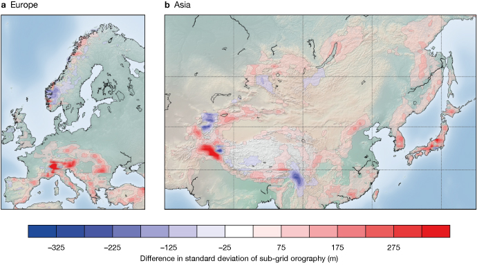
The next step is to try to optimise directly the parameters of the sub-grid scale orography parametrization instead of the well-known standard deviation of sub-grid orography. This parameter estimation step can be performed either using machine learning techniques offline, or directly inside the 4D‑Var minimisation.
Bias correction of observations
Observational bias correction might be a good application for machine learning. If we knew the physical explanation for a bias, we would correct it at source in the forecast model or observation operator. But it is often difficult to find physical explanations for biases between the simulated observations and their real equivalents, so biases are often corrected using empirical models. In the IFS, variational bias correction (VarBC) is one example. Currently it only allows linear bias models as a function of predictors like layer thickness, skin temperature or satellite viewing angle. Nonlinear models can be added in VarBC by using linearising transforms, such as terms from the Fourier transform or a polynomial expansion. The latter is already used with the satellite scan angle. However, these transforms are only capable of fitting some nonlinear behaviours. For a completely free-form nonlinear empirical fit, a neural network could be a good alternative. It might even be possible to use a neural network as a bias model within VarBC, although that has not yet been tested. On the other hand, a neural network with a single layer and a linear activation function is just an offline version of VarBC, in other words they both simplify to multiple linear regression.
We show an example using an offline neural network bias correction applied to the solar-dependent bias of the Special Sensor Microwave Imager/Sounder (SSMIS). This varies through the orbit and through the year in a complex pattern (Figure 4a). The red arches near the bottom of the plot are the most difficult part: at certain times of the year, the instrument calibration changes rapidly as the satellite emerges from the dark into the sunny part of the orbit. VarBC absorbs some of this bias but cannot deal with these sharp features (not shown). However, VarBC has the advantage of being able to evolve through time, following the changing bias as the satellite’s orbit drifts. The difficulty of applying a neural network is, first, that there is a lack of training data: one year’s bias cycle is just a single training point; second, it would need to be continually re‑trained to keep up with the evolving bias; in machine learning it is more typical to train once and then use a fixed network for prediction.
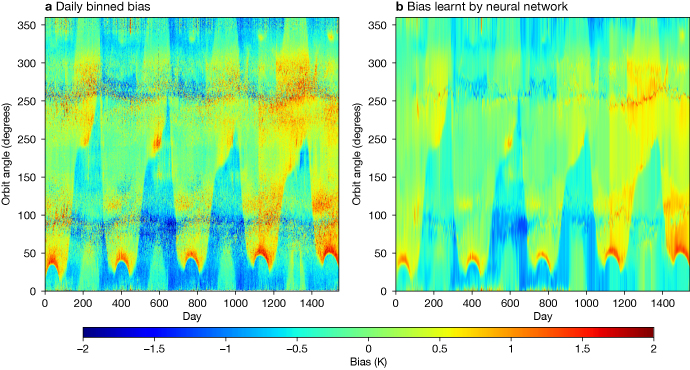
Figure 4b shows a simple adaptation, where the neural network is only expected to predict the bias one day ahead, and it is re-trained every day on the new day’s data, so that it slowly adapts. The neural network produces a smooth fit to the strongly nonlinear variations in bias through the orbit. With the cycled training, it can also evolve through time. This is an example of ‘transfer learning’, where a pre-trained neural network is re‑trained on new data. However, standard machine learning is only just starting to evolve the tools to control the learning rate of such a network, in other words to control how fast it evolves. Further, it is hard to specify how much of the information gets fitted; the big worry with VarBC has always been that, with too many degrees of freedom, useful observational information could end up being aliased into the bias correction rather than being used, as intended, to update the initial conditions.
To move from multiple linear regression towards a free-form nonlinear empirical model is just a possible evolution for VarBC. There is no binary choice between ‘data assimilation’ or ‘ML’. The real issues are more technical: whether the solver in 4D‑Var is capable of fitting a neural network embedded in 4D‑Var (or whether quick gains could be made with an offline neural network of the type explored here); how to constrain the shape of the empirical fit so that useful observational information goes into the atmospheric state analysis and not the bias model; and how to constrain the evolution of the bias model through time. These issues are equally relevant for any data assimilation or ML approach.
Outlook
From a data assimilation perspective, ML/DL does not introduce completely new or revolutionary ideas. As we have shown here, ML/DL techniques have much in common with the standard workflow of variational data assimilation, though these similarities tend to be partly obfuscated by the different nomenclature used in the two fields. These similarities make it conceptually easy to integrate standard ML/DL techniques and ideas into the 4D‑Var workflow. However, the practical and technical challenges, e.g. arising from the use of different programming languages or the difficulties associated with developing and deploying online ML/ DL algorithms, should not be underestimated. We have shown some concrete initial examples of how this can be done in the IFS, focussing on improving and correcting the models used in the data assimilation cycle. There are obviously many other possibilities and application areas in the whole NWP workflow (as discussed in Düben et al., 2021). As the number of possible developments at the intersection of data assimilation and machine learning is vast, collaborations with the broader research community from both Member and Co‑operating States and academia is crucial to accelerate the pace and quality of developments. An example of this type of collaboration is the joint work with ECMWF Fellow Marc Bocquet and his group at the École des Ponts ParisTech, which has already resulted in significant insights on how to more closely embed machine learning techniques in the data assimilation system for the estimation and correction of model errors (Farchi et al., 2021).
More generally, the most recent ML/DL wave of interest has brought into renewed focus the opportunities offered by data-driven techniques to improve and/or correct our knowledge-based models, thanks to the huge and ever-increasing amount of accurate Earth system observations available for NWP and climate prediction initialisation. However, for reasons discussed in e.g. Bonavita & Laloyaux (2020), while it is clear that these tools can be useful complements and additions to our physics-based models, it would be naïve to believe that they can replace them entirely.
Further reading
Bonavita, M. & P. Laloyaux, 2020: Machine learning for model error inference and correction. Journal of Advances in Modeling Earth Systems, 12, e2020MS002232. https://doi.org/10.1029/2020MS002232.
Düben, P., U. Modigliani, A. Geer, S. Siemen, F. Pappenberger, P. Bauer et al., 2021: Machine Learning at ECMWF: A Roadmap for the next 10 years. ECMWF Technical Memorandum No. 878. https://doi.org/10.21957/ge7ckgm.
Farchi, A., P. Laloyaux, M. Bonavita & M. Bocquet, 2021: Using machine learning to correct model error in data assimilation and forecast applications, Quarterly Journal of the Royal Meteorological Society (under review).
Geer, A.J., 2021: Learning earth system models from observations: Machine learning or data assimilation?, Phil. Trans. R. Soc. A, 379: 20200089. https://doi.org/10.1098/rsta.2020.0089.
Laloyaux, P. & M. Bonavita, 2020: Improving the handling of model bias in data assimilation. ECMWF Newsletter No. 163, 18–22.