ECMWF aims to analyse the full state of the Earth system from the atmosphere and ocean through to the land surface and cryosphere. This is intended to be achieved through closer coupling of the relevant models and the data assimilation systems that combine the model forecasts with new observations. But aspects of the Earth system, such as sea ice, snow, soil and vegetation, are hard to model from physical first principles, so in practice, the modelling can be quite empirical. Earth system modelling components are often parametrized or fitted based on a limited set of observations from experimental ground stations, and they may struggle to perform in other locations. A ‘model first’ approach has served us well in the atmosphere, where at least the dynamics are mostly well known: here the purpose of observations is to correct the physical trajectory of the model. But the recent explosion in machine learning for Earth system applications has shown us an ‘observation first’ approach. If observation-driven machine learning forecasts are starting to do better than physical forecasts, it suggests we have not been making good enough use of observations to improve our forecast models. Especially for Earth system applications where models are already partly empirical, there is clearly great potential to let the observations increasingly define these models. However, as demonstrated in this article with the example of sea ice assimilation, the best results are unlikely to come by throwing away physical models entirely, but by carefully combining known physics with empirical components.
Getting more out of satellite observations
Taking a global viewpoint, available observations of the Earth system come mainly from satellites, and primarily from the naturally-generated radiation that is emitted by the Earth. An observational viewpoint starts from understanding what information the measured radiances contain and how to extract that information into useable geophysical variables. If we take microwave observations as an example (Figure 1), we can see by eye the overlapping sensitivities to the atmosphere (clouds, precipitation, water vapour, temperature) and the surface (ocean surface state, sea ice and its snow cover, snow, vegetation and soil moisture). The atmospheric sensitivities are currently used in all-sky radiance assimilation within ECMWF’s 4D-Var atmospheric data assimilation. But the surface sensitivities remain mostly unused, in part due to the difficulty of physical modelling. These difficulties concern both the forecast model for the surface state and the translation between the surface state and the observations, which is done by the observation operator (sometimes called an observation model). The goal of making full use of the information contained in these observations is often described as ‘all-sky, all-surface assimilation’.

A better use of the information in satellite observations has three benefits:
- we get more information on the atmospheric state in areas where satellite observations were previously discarded, such as sea ice, snow and land surfaces
- we get new information on poorly known variables, such as sea ice concentration, snow cover or soil moisture
- we can use the observations to help constrain, improve and develop better physical and empirical models of the Earth system.
The contention of this article is that we will make the furthest progress in the middle ground between model-led approaches and purely observation-driven approaches. Traditional data assimilation frameworks and newer machine learning approaches alike are best understood as Bayesian problems (see Box C later). What this means is that we aim to maximise the information extracted from current observations while making best use of our prior information, whether that comes from physical laws or from historical observations. This is not only a theoretical argument. A middle-ground, Bayesian-inspired approach is already helping us make rapid progress towards better use of surface-sensitive observations in our operational weather forecasting system. The example here is sea ice, but the same techniques can be used across the Earth system. The question is not whether to use physical or empirical models, but how best to combine them.
The sea ice problem
Sea ice is an attractive first target for approaches that combine machine learning and data assimilation. It is also a perfect illustration of how we can get more out of satellite observations while retaining physical modelling where possible. It covers all three areas where we would expect benefits:
Get more information on the atmosphere: In the current atmospheric 4D‑Var, we have to reject any satellite observations with strong sensitivity to sea ice. As a result, there is a particularly severe information desert in southern hemisphere high latitudes. As will be illustrated in this article, putting more observations into this desert results in significant forecast improvements.
Get more information on the surface: Microwave radiance observations are already used in the ECMWF sea ice analysis. The problem is that they are finally introduced into the atmospheric analysis by a slow, roundabout, and sub-optimal route. Sea ice concentration retrievals are inferred using heuristic approaches, then incorporated into a daily analysis at the UK Met Office, then assimilated into ECMWF’s OCEAN5 system, then passed to the atmospheric data assimilation with an overall delay of around 48 hours. If we can use our in-house data assimilation tools to infer the sea ice concentration directly from the radiances, we can eliminate the delay and almost certainly do a better job of inferring the state of the sea ice, too.
Use the observations to develop better physical and empirical models of the Earth system: One reason the sea ice analysis is still so far behind the atmosphere is a lack of accurate enough physical models, both to propagate the state forward in time and to model the radiance observations. In particular, the state variables that affect the radiative transfer properties of sea ice include aspects of the microstructure of the ice and snow that are not represented in current physical models.
This final aspect makes the problem just as challenging from a machine learning perspective as for data assimilation. The normal machine learning approach, known as ‘supervised learning’ (we might also call this ‘brute force’), attempts to learn an empirical model given its known inputs and outputs. For the sea ice observation problem, we know the outputs – these are the satellite radiance observations – but the inputs, including the microstructural details of the ice and snow, are basically unknown in the absence of ice core and snow pit measurements. This is a chicken and egg problem, and its solution starts by acknowledging that we need to simultaneously learn the state of the sea ice and the empirical observation model to go from that to the observations. The problem is solved by combining both data assimilation and machine learning in a Bayesian framework with parallels to ‘unsupervised’ or ‘generative’ machine learning techniques.
To practically solve this problem, a year’s worth of microwave radiance observations were paired with atmospheric profiles from the background (short-range) forecast of the Integrated Forecasting System (IFS). Machine learning tools built on top of Python, Keras and Tensorflow were used to set up a hybrid data assimilation and machine learning framework to simultaneously learn the sea ice state along with an empirical model for the sea ice surface emissivity. Here the surface emissivity is a convenient way of representing the surface radiative transfer. Unlike standard data assimilation frameworks used for real-time forecasting, this offline approach was able to simultaneously fit a whole year of observations in one go.
Box A and its figure illustrate the resulting empirical-physical model as it applies to the surface radiative transfer for one observation. It takes physical inputs, namely the sea ice concentration, the skin temperature, and the ocean water surface emissivity, and three empirical inputs that represent the microstructural and physical state of the sea ice and the snow on top of it. It outputs the surface emissivity of the combined ocean and sea ice scene observed by the satellite. Because of the simple physics encoded in the network, it is capable of being used to infer physical variables, namely the sea ice concentration.
A
The physical-empirical model
The figure shows the key part of the empirical-physical Bayesian network used for learning the sea ice state and the empirical model for the sea ice surface emissivity. The complete model component describes the mixed-surface emissivity within the field of view of a single satellite observation. Here bold outlines are independent variables, with solid outlines if they are held fixed (obtained from the ECMWF background forecast) and dashed outlines if they are to be estimated within the learning framework. Fine outlines indicate variables that are just dependent functions of other variables. The empirical part of the model estimates the sea ice surface emissivity based on the skin temperature and three empirical variables representing the state of the sea ice and the snow cover on top of it (more of this in Box B). In practice, the empirical model is a simple one-layer linear neural network, though deep nonlinear neural networks have also been trained in this framework but proved unnecessary. The physical part of the model represents the mixed surface emissivity as a linear weighted combination of the ocean surface emissivity and the sea ice surface emissivity. It is this physical emissivity contrast between sea ice and open ocean surfaces that ultimately allows the sea ice concentration to be estimated within the field of view of a satellite observation.
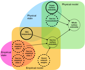
The broader network, not shown here, holds daily maps of the four learned state variables. It offers interpolation operators to go from the maps to the observation time and location, so that in reality it is the maps that are the true trainable variables, not the observation-space variables as shown here. The neural network weights are the same throughout the year and at all locations, with the aim to create a universally valid empirical model for the sea ice surface emissivity. The mixed surface emissivity is input to a physical radiative transfer model that represents the atmosphere including clouds and precipitation (obtained from the ECMWF background forecast). The aim of the training is to find the maps of surface state and the neural network weights that will generate simulated observations that best fit a year’s worth of real observations. The training is done simultaneously on all observations using the variational inverse Bayesian framework common to both machine learning training and 4D‑Var data assimilation.
This same network fragment is extracted, along with the trained network weights, to be implemented in operational 4D‑Var as part of the observation operator for all-sky, all-surface microwave observations. In 4D‑Var, the learnable input variables are estimated at observation locations, but keeping the neural network weights fixed.
The quality of the resulting sea ice concentration analysis is illustrated in Figure 2 during the rapid freeze-over of the Arctic ocean during November 2020. The OCEAN5 sea ice analysis represents the Siberian side of the Arctic ocean as open water, due to the 48‑hour delay, whilst the new approach shows that it has already mostly frozen over. The new empirical-physical model is also able to closely replicate microwave observations at frequencies from 10 GHz to 89 GHz, in all seasons and both in the Antarctic and the Arctic (not shown).
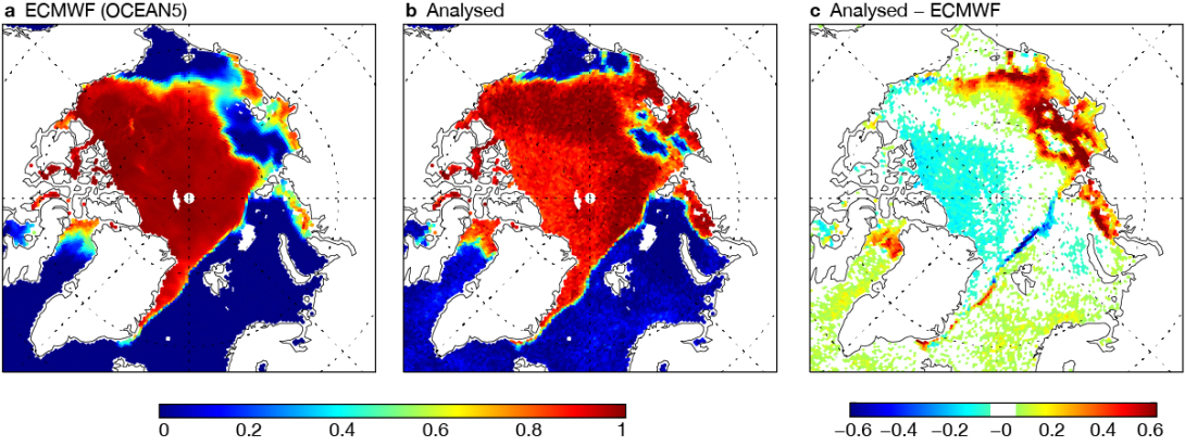
The empirical variables representing the detailed microstructural and physical aspects of the sea ice and snow state are explored in Box B.
B
The empirical state variables
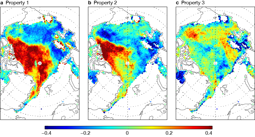
The simultaneous training of an empirical state alongside an empirical model is what allows us to solve the chicken and egg problem. The figure shows maps of the empirical ice properties on 7 November 2020, the same date as the sea ice maps in Figure 2. Empirical property 1 follows known differences between multi-year and first-year ice. The positive (red) values are found in areas of long-lived ice. The negative values (blue) correspond to areas where the sea ice is newly formed. New ice contains pockets of brine. This is lost over subsequent months, leaving behind air pockets that strongly scatter microwave radiation. At higher microwave frequencies, the microstructural characteristics of the snow lying on top of the sea ice become most important. The second and third empirical properties help represent this and other aspects of the sea ice and snow properties that affect the radiative transfer.
The offline analysis of the sea ice state and observation model is on one hand an illustration of how the Bayesian approach could be used, along with empirical state variables where required, to solve all our Earth system problems using an observation-first perspective. On a more practical level, it is also a first step in adding sea ice assimilation to the IFS.
Assimilating sea ice observations in the IFS
From the offline machine learning and data assimilation framework, we have a model (Box A) that can be plugged into the existing atmospheric 4D-Var framework of the IFS. This becomes part of the observation operator alongside the existing RTTOV (Radiative Transfer for TOVS) model for the radiative transfer of the atmosphere including clouds and precipitation. To estimate the four poorly-known model inputs, namely the sea ice concentration and the three empirical variables, 4D-Var uses an observation-space augmented control vector similar to the ‘skin temperature sink variable’ that has been used in satellite data assimilation at ECMWF for several decades. So, as well as estimating the state of the atmosphere in the usual way, 4D-Var also estimates the sea ice concentration and the three empirical variables at each observation location from microwave imager observations, namely the Advanced Microwave Scanning Radiometer 2 (AMSR2) and the GPM microwave imager (GMI).
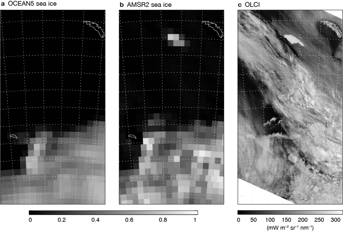
An illustration of the quality of the resulting 4D-Var sea ice concentration analyses is provided by Figure 3. During the autumn and winter of 2020, the giant iceberg A-68A was drifting from its source in the Weddel sea and came close to the Southern Ocean island of South Georgia. At the time, A-68A was being tracked visually using radar and visible measurements, but the new sea ice analysis in 4D-Var has made a retrospective track of its movements that agrees well with the contemporary analysis. The figure shows A-68A approaching South Georgia on 4 December. At around 100 km long and 60 km wide, the iceberg is of similar size to the island itself. Allowing for the fact that the observation-space sea ice analysis has a relatively coarse resolution of around 40 km, it shows very similar features to the visual picture from the OLCI sensor on Sentinal-3. By contrast, the OCEAN5 analysis does not represent the iceberg.
Benefit of sea ice observations for atmospheric forecasts
Figure 4 shows the impact of adding microwave observations in sea ice areas on the temperature forecast, based on year-long testing in 2021 and 2022. Notably, this testing period is different to the training period used in the offline machine learning framework, which was 2020 to 2021. The new observations over sea ice areas have little impact on the Arctic forecast, likely because the year-round availability of in-situ measurements helps fill any gaps in the satellite data. But in the Southern Ocean, particularly around 50 to 60 degrees south, there is a statistically significant improvement in the forecast that lasts out to around day 4 and that spans from the surface up to the mid-troposphere. This localised impact is strong enough to also generate a statistically significant improvement in the headline southern hemisphere (20°S to 90°S) forecast scores.
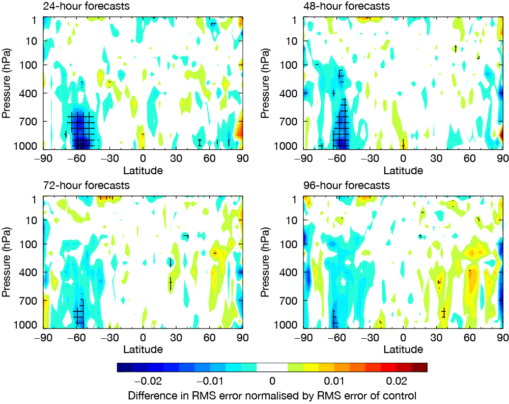
Figure 5 shows the number of observations being assimilated in atmospheric 4D-Var in IFS Cycle 48r1 (control) and experimental IFS Cycle 49r1 (sea ice) from the AMSR2 sensor during June 2022. The added observations in the Arctic are limited to the relatively small area of summer sea ice. By contrast, a much larger area of the Southern Ocean, including both the sea ice and its surrounding areas, gains microwave imager observations for the first time. The new sea ice assimilation has relatively large observation errors and the added ‘safety valve’ of being able to adjust the surface emissivity to fit the observations. A side effect is that it is possible to assimilate for the first time ‘cold air outbreak’ regions over the ocean in the vicinity of the sea ice (Forbes et al., 2016). It appears that most of the atmospheric forecast benefit comes from these new observations, rather than those over the sea ice itself. However, as the modelling improves and observation errors are reduced in future years, it is expected that observations over sea ice will provide atmospheric information, too.
A further detail of Figure 5 is that the density of observations is up to six times higher in the polar regions than at midlatitudes. This is due to the polar sun-synchronous orbit used by most meteorological satellites, which in this case takes the AMSR2 sensor over part of each polar cap every 100 minutes. Further development of the sea ice and snow analysis could release a huge amount of high temporal frequency data from polar-orbiting satellites in polar regions.
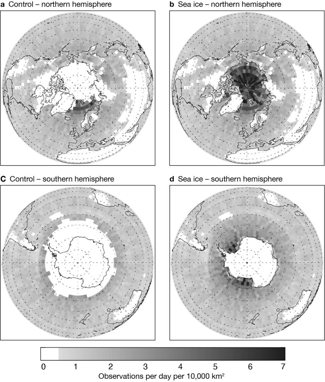
FIGURE 5 Number of observations per day per 10,000 km2 assimilated from AMSR2 (in its 37 GHz v-polarized channel) between 1 June and 5 June 2022 in (a) the Cycle 48r1 control configuration in the northern hemisphere, (b) the Cycle 49r1 sea ice configuration in the northern hemisphere, (c) the Cycle 48r1 control configuration in the southern hemisphere, and (d) the Cycle 49r1 sea ice configuration in the southern hemisphere.
Future developments
The sea ice assimilation described in this article is intended to become operational with Cycle 49r1 of the IFS in the middle of 2024. For the moment, the main practical benefit will be improved forecasts in the Southern Ocean. But the next stage of development is to assimilate the sea ice concentration analyses into the ocean data assimilation component using an outer-loop coupling data assimilation framework. This will also assimilate new sea-surface temperature (SST) retrievals from the microwave observations, testing an approach that could ultimately eliminate the need to use external SST and sea ice concentration (SIC) products in the ocean analysis, along with the 48‑hour delay this entails. That next stage is in development and will be documented elsewhere.
The techniques that have enabled us to get started with sea ice assimilation are also immediately applicable to snow over land and, with further development, the whole land data assimilation problem, including soil moisture and vegetation. There is scope to extend the empirical-physical modelling to a wider range of microwave frequencies and viewing geometries, aiming to start assimilating not just microwave imaging channels over sea ice (10 to 89 GHz) but also microwave sounding channels, which provide a leading contribution to forecast accuracy over surface types that are easier to assimilate. One aim is to move the surface radiative transfer modelling away from the use of surface emissivity and towards a more physical representation of scattering and absorption within the sea ice and snow pack. And when improved forecast models of sea ice and snow are coupled into atmospheric 4D‑Var, the empirical modelling can be re-trained using these additional physical inputs. The long-term aim is to increasingly impose physical constraints and to minimise the use of empirical models and empirical state variables.
For an even wider perspective, we can go back to the Bayesian viewpoint that unifies machine learning and data assimilation. It is this framework that makes the hybrid sea ice state and model estimation possible, and this framework will lie behind its future extensions into the whole area of Earth system data assimilation. The Bayesian approach treats both prior knowledge and observations in a theoretically correct way. This means we can obtain the best possible information on the current state of the Earth system and its modelling components (see Box C). Prior knowledge can be encoded using the physical equations of the Earth system that we already know. But we can also encode the areas of the Earth system that we know less well using empirical model components that can be learned from observations.
C
The Bayesian approach
Bayes’ theorem comes out of fundamental rules of statistics and shows how to combine prior information with new observations to gain an improved knowledge of the world. Bayes’ theorem is formulated in terms of ‘prior’ and ‘posterior’ probability distribution functions and is hard to solve directly for high-dimensional problems like the Earth system. Variational data assimilation turns Bayes’ theorem into a tractable method for ingesting observations by using the assumption of Gaussian error distributions. But the applications of Bayes’ theorem are far wider, both philosophical and practical. One key extension is the ‘Bayesian network’, which enables us to break up huge probabilistic problems into simpler components if we know (or can learn) the statistical dependencies between variables. The hybrid empirical-physical model in Box A is also an illustration of the Bayesian network describing sea ice and ocean surface radiative transfer, where the arrows represent the dependencies, and the circles represent statistical variables. Again, it is solved by making simplifying assumptions and by doing a variational minimisation to fit new observations, just like 4D-Var or indeed most neural network training. Within these networks, known physics can be represented using fixed physical equations. Unknown physics, such as the sea ice surface emissivity, can be represented using an empirical model such as a neural network. Typical ‘brute force’ machine learning throws away all the prior physical knowledge and attempts to learn from the new observations alone. Unless these observations contain all knowledge, then by Bayes’ theorem, brute force machine learning cannot possibly provide as much posterior knowledge of the world as we can gain by using a learning process that includes prior knowledge.
If we could completely implement the Bayesian network framework, it would help us balance the information gleaned from the limited field measurements that underpin many current Earth system parametrizations with the vast and continuing amount of information coming from satellite observations. It would help us derive much more sophisticated physical parametrizations that would work more universally across the globe. The role of the scientist would move away from finding heuristic or regression models based on limited field observations. Instead, the job would be to encode the physics we already know, to correctly describe our confidence in this knowledge, and to make sure that Earth observations are used as completely as possible. This is not just an issue for the ‘newer’ aspects of Earth system studies, such as sea ice, snow or vegetation, but for the ‘older’ empirical aspects of atmospheric models, such as cloud and precipitation parametrizations and sub‑grid scale physics. Although it would be a daunting task to break apart our current systems and re‑implement them in a unified Bayesian framework, many of the tools already exist and are being used for machine learning; indeed, they underpin its current success.
In comparison to a brute-force machine learning approach, a careful hybrid of the physics we already know with all the new and evolving knowledge that comes from observations will always give us a better understanding, not just of the Earth system state but also the physical and empirical models that represent its evolution. It is only in a few places in the world, such as at ECMWF, that all the different components of observations, prior physical knowledge, and Bayesian learning methods (including data assimilation and machine learning) can be brought together to generate the highest-quality Earth system analyses and forecasts.
Further reading
de Rosnay, P., P. Browne, E. de Boisséson, D. Fairbairn, Y. Hirahara, K. Ochi et al., 2022: Coupled data assimilation at ECMWF: Current status, challenges and future developments, Q. J. R. Meteorol. Soc., 148, 2672–2702. https://doi.org/10.1002/qj.4330
Forbes, R., A. Geer, K. Lonitz & M. Ahlgrimm, 2016: Reducing systematic errors in cold-air outbreaks, ECMWF Newsletter No. 146, 17–22. https://doi.org/10.21957/s41h7q7l
Geer, A.J., 2021: Learning earth system models from observations: machine learning or data assimilation? Phil. Trans. R. Soc. A, 379. https://doi.org/10.1098/rsta.2020.0089
Geer, A.J., 2023: Simultaneous inference of sea ice state and surface emissivity model using machine learning and data assimilation (in preparation).
Geer, A.J., 2023: Joint estimation of sea ice and atmospheric state from microwave imagers in operational weather forecasting (in preparation).
